
|
While not nearly as powerful as a statistical computing environment like R, Excel offers the advantage of being able to be found in just about every work environment. As such, knowing how to do statistical calculations and simulations in Excel can be very useful.
Rather than using named variables to store values to be used later, like one might see in R or any other programming languages, Excel stores values it needs for subsequent calculations in cells. Each cell is part of a particular worksheet and has a unique row/column combination in that sheet. The row is indicated by a positive integer and the column is indicated by a letter (or sequence of letters if more than 26 letters need be used).
An example worksheet is shown below.
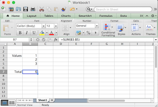
Notice in the sheet above cells B3, B4, and B5 contain numerical values, while cells A3 and A7 contain text.
There are other things that cells can contain as well. B7 looks like it contains a value, but clicking on it reveals that the content of the cell is actually a formula, and the value shown is simply the output of that formula.
In this case, the formula finds the sum of the range of all cells between B3 and B5, inclusive and is given by: "=SUM(B3:B5)". This formula can be seen by selecting cell B7 and then looking at the text-edit box with a $fx$ to its left in the tool bar at the the top. Importantly, one should know that all formulas begin with "=", followed by some expression.
The expression B3:B5 in the formula above specifies a range of cells. Using ranges allows one to efficiently make calculations even if they involve large amounts of data.
In general, a range takes the form of two cell addresses separated by a colon (":"). These two cells are typically the upper left and lower right cells of some rectangular collection of cells, although they may also be the lower left and upper right cells of the same.
The use of "SUM()" in the aforementioned formula specifies what function to apply to the range(s) of cells it is given as arguments inside the parentheses to the right of the function's name. Excel has a huge number of built-in functions that can be used to a great variety of ends. To see what it has to offer, click the "$fx$" button in the toolbar at top to bring up the formula builder dialog box. Clicking on a particular function name brings up more information on what the corresponding function calculates, the proper syntax for using it (i.e., how to type it correctly), and a link to even more information on the function.
The left side of the worksheet shows an example of using the AVERAGE() function on the range of cells given by B3:F5
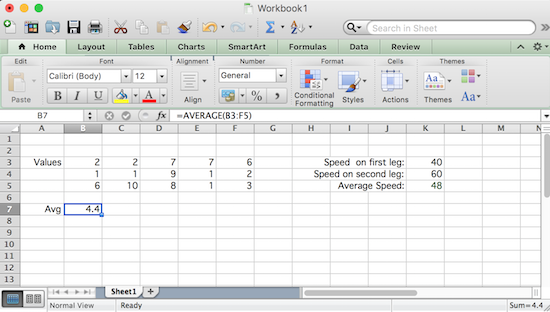
Formulas can also reference individual cell values, as the right side of the worksheet above demonstrates. If we clicked on cell K5, we would see "=2/(1/K3+1/K4)", the formula for the harmonic mean of the values seen in cells K3 and K4. When using mathematical expressions in a formula in Excel, the standard order of operations applies. Consequently, given that we must enter these expressions using a single line of text, one needs to be careful. A very common mistake is forgetting to group numerators, denominators, or even some exponents with parentheses, when their inclusion is necessary.
There are a couple of "tricks" in Excel that one can use to quickly flesh out a range of cells...
The first is that Excel supports a relatively intelligent "autofill". Suppose you wanted to quickly create a column of cells from 1 to 10. Simply type the values for the first two cells, and then select these cells, noting the small square "handle" at the bottom right corner of that selection.
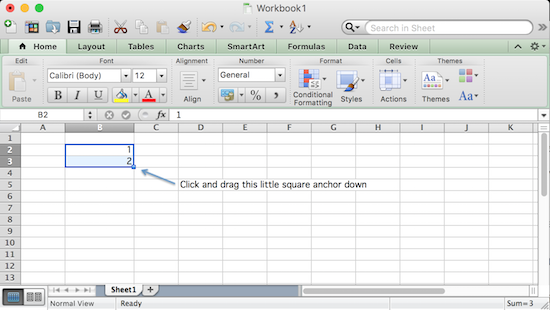
Want the sequence $3,5,7,9,\ldots$ instead? Simply start with 3 and 5 as your first two cells, and drag down as before -- Excel will figure out what you want and fill the cells accordingly. This process works for any linear sequence.
Another trick that can really save you time when filling a range of cells is the use of an "anchor". To set the stage for understanding what an anchor is, consider the following...
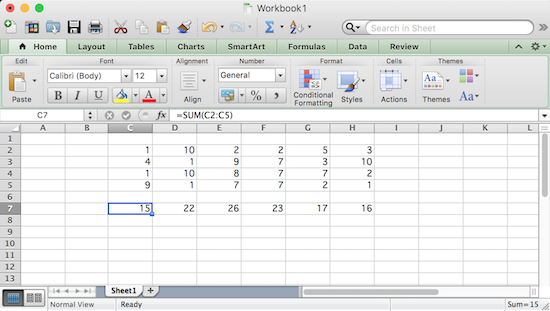
The RANDBETWEEN() function generates a random integer between the two arguments it is provided. Suppose we enter the formula "=RANDBETWEEN(1,10)" in cell C2 to generate a random integer between $1$ and $10$ in this cell, and then copy the content of this cell to all of the cells in range C3:H5 to create six columns of random numbers similar to what is shown below.
Now suppose we wish to sum the various columns. If we enter "=SUM(C2:C5)" in cell C7 to sum the numbers in column C, and copy that formula to cells in the range D7:H7, we get correct column totals for each column.
This works because when one copies a formula to another cell, the cell references are updated in a relative way. As a simple example of this relative addressing -- if a formula in cell A1 references B1, the cell to its immediate right, and is copied to cell J5 for instance, then the former reference to B1 is changed by Excel to reference the cell K5, the cell to J5's immediate right.
Anchors allow us to change this default behavior when copying formulas to other cells, so that anything that has been "anchored" doesn't get updated due to the change in relative position.
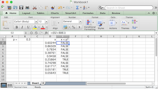
As an example, suppose one wanted to generate 10 simulations of a game that one had a 30% chance of winning. They also wanted their work to be flexible enough so that it could be easily adapted to a different chance of winning.
We start by putting the text of "p = " in cell A1, followed by the value 0.30 in B1 to indicate the probability of winning the game. We also put the text "x" and "x < p?" in cells D1 and D2, respectively, as column headers for the part coming up...
Then, noting that the RAND() function generates a random value between $0$ and $1$, we enter "=RAND()" in cell D2, select it, and use the handle to autofill this formula to the 9 cells below it.
To use these numbers to simulate a win or loss, in cell E2, we enter "=(D2<$B$1)". This will return a "value" of TRUE or FALSE depending on whether or not the value of cell D2 is less than that in B1, as appropriate. In this way, every TRUE produced represents a win and every FALSE represents a loss.
You may be wondering about the presence of the two dollar signs in the $B$1 just used. This is the "anchor" previously mentioned. When we copy the formula in cell E2 to lower cells, we want to make a comparison between the value of the cell to the immediate left of the cell in column E and in its same row (relative addressing), and the value of the cell B1, regardless of which row in E we are on. The presence of the dollar signs essentially says: "When this formula is copied to another cell, the row or column references after each dollar sign won't be changed." Using them in this way is known as absolute addressing.
With all of the cells making comparisons with the single cell B1, if one wished to change the probability of winning the game to 50%, all one would need do is change the value in that cell to 0.5.
The reason we need two dollar signs instead of a single one in our formula, is that Excel lets one anchor the rows and columns independently. The presence of the dollar sign in front of the row value anchors only the row, while the presence of the dollar sign in front of the column letter(s) anchors only the column.
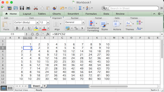
This independence between row and column anchors can be particularly helpful when creating a table of values that depend on two inputs. For example, consider creating a simple multiplication table. We fill cell C2 and D2 with values 1 and 2 and autofill to the right to create the column headers of our table. In a similar manner we create row headers in the range B3:B12. Then, to create the body of the table, we simply type "=$B3*C$2" in cell C3 and copy it to the rest of the cells in the range C3:L12. (Think carefully about why this works!)
As one more trick -- suppose you wish to copy a cell to a large range. You can of course copy the cell and then manually select the large range, but this might require a lot of scrolling if the range involves thousands of rows or columns. Instead, one can select a large group of cells for copying, pasting, or other needs, by going to the "Edit" menu, and selecting "Find : Go To" from there. At that point, enter the range that you wish to select in the blank marked "Reference" and click "OK". The large range is now selected! Note: Ctrl-G or F5 can be used is a keyboard shortcut to bring up the "Go To" dialog box, to speed up the selection process even further.
Usefully, one can use formulas to fill a range with a recursively defined sequence.
For example, the Fibonacci sequence $1, 2, 3, 5, 8, 13, \ldots$ is the sequence that begins with $1, 1$, with later terms each being the sum of the two terms that precede it.
Notice how easy it is to create this sequence in Excel, as shown below.
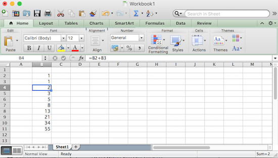
Here, we first enter 1 in cells B2 and B3, and then enter the formula "=B2+B3" in cell B4. Then -- letting relative addressing do its work -- either copy or autofill this formula to the cells below it, to obtain the sequence shown.